from statsmodels.tsa.ar_model import AR
from statsmodels.tsa.arima_model import ARIMA
from statsmodels.graphics.tsaplots import plot_acf, acf
from statsmodels.tsa.stattools import adfuller
from statsmodels.graphics.tsaplots import plot_pacf
from statsmodels.tsa.stattools import adfuller

import pandas as pd
import matplotlib.pyplot as plt
import numpy as np
from warnings import filterwarnings
filterwarnings("ignore")

데이터 불러오기 (pd.read_csv)
python 파일 경로에 만든 후 data5폴더에 다음의 'daily-total-female-births.txt' 파일 넣어놓기
# ,로 되어있으면 csv로 읽으면됨(txt파일이라도)
birthDF = pd.read_csv('data5/daily-total-female-births.txt',
                      parse_dates=['Date'], index_col='Date') # parse_dates=['Date'] : Datetime으로 형변환
birthDF

birthDF.index[OUT] :
DatetimeIndex(['1959-01-01', '1959-01-02', '1959-01-03', '1959-01-04',
'1959-01-05', '1959-01-06', '1959-01-07', '1959-01-08',
'1959-01-09', '1959-01-10',
...
'1959-12-22', '1959-12-23', '1959-12-24', '1959-12-25',
'1959-12-26', '1959-12-27', '1959-12-28', '1959-12-29',
'1959-12-30', '1959-12-31'],
dtype='datetime64[ns]', name='Date', length=365, freq=None)
birthDF.info()[OUT] :
<class 'pandas.core.frame.DataFrame'>
DatetimeIndex: 365 entries, 1959-01-01 to 1959-12-31
Data columns (total 1 columns):
# Column Non-Null Count Dtype
--- ------ -------------- -----
0 Births 365 non-null int64
dtypes: int64(1)
memory usage: 5.7 KB데이터 불러오기 (pd.read_csv)
python 파일 경로에 만든 후 data5폴더에 다음의 'international-airline-passengers.txt' 파일 넣어놓기
airDF = pd.read_csv('data5/international-airline-passengers.txt',
                   parse_dates=['time'], index_col='time')
airDF

airDF.info()[OUT] :
<class 'pandas.core.frame.DataFrame'>
DatetimeIndex: 144 entries, 1949-01-01 to 1960-12-01
Data columns (total 1 columns):
# Column Non-Null Count Dtype
--- ------ -------------- -----
0 passengers 144 non-null int64
dtypes: int64(1)
memory usage: 2.2 KB
airDF.index[OUT] :
DatetimeIndex(['1949-01-01', '1949-02-01', '1949-03-01', '1949-04-01',
'1949-05-01', '1949-06-01', '1949-07-01', '1949-08-01',
'1949-09-01', '1949-10-01',
...
'1960-03-01', '1960-04-01', '1960-05-01', '1960-06-01',
'1960-07-01', '1960-08-01', '1960-09-01', '1960-10-01',
'1960-11-01', '1960-12-01'],
dtype='datetime64[ns]', name='time', length=144, freq=None)데이터 불러오기 (pd.read_csv)
python 파일 경로에 만든 후 data5폴더에 다음의 'daily-min-temperatures.csv' 파일 넣어놓기
tempDF = pd.read_csv('data5/daily-min-temperatures.csv',
                   parse_dates=['Date'], index_col='Date')
tempDF
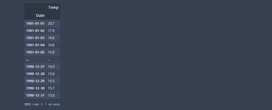
tempDF.index[OUT] :
DatetimeIndex(['1981-01-01', '1981-01-02', '1981-01-03', '1981-01-04',
'1981-01-05', '1981-01-06', '1981-01-07', '1981-01-08',
'1981-01-09', '1981-01-10',
...
'1990-12-22', '1990-12-23', '1990-12-24', '1990-12-25',
'1990-12-26', '1990-12-27', '1990-12-28', '1990-12-29',
'1990-12-30', '1990-12-31'],
dtype='datetime64[ns]', name='Date', length=3650, freq=None)
tempDF.info()[OUT] :
<class 'pandas.core.frame.DataFrame'>
DatetimeIndex: 3650 entries, 1981-01-01 to 1990-12-31
Data columns (total 1 columns):
# Column Non-Null Count Dtype
--- ------ -------------- -----
0 Temp 3650 non-null float64
dtypes: float64(1)
memory usage: 57.0 KB
birthDF.plot()
plt.show() # stationary

airDF.plot()
plt.show() # non-stationary

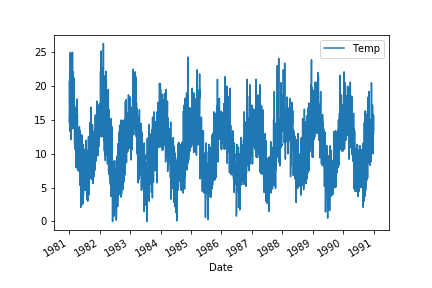
tempDF.plot()
plt.show()
# stationary? non-stationary? 평균과 분산은 일정해보이지만 주기성을 가지고 있다 -> 판별해보자
# 보통 주기를 가지고 있으면 non-stationary
stationary
# 반을 나눠서 앞뒤 평균분산 확인 -> 차이 얼마 안남
n = int(len(birthDF)/2)
print(birthDF.iloc[:n].mean())
print(birthDF.iloc[n:].mean())
print(birthDF.iloc[:n].var())
print(birthDF.iloc[n:].var())
[OUT] :
Births 39.763736
dtype: float64
Births 44.185792
dtype: float64
Births 49.485308
dtype: float64
Births 48.976281
dtype: float64non-stationary
# 반을 나눠서 앞뒤 평균분산 확인 -> 차이 많이남(non-stationary)
n = int(len(airDF)/2)
print(airDF.iloc[:n].mean())
print(airDF.iloc[n:].mean())
print(airDF.iloc[:n].var())
print(airDF.iloc[n:].var())
[OUT] :
passengers 182.902778
dtype: float64
passengers 377.694444
dtype: float64
passengers 2275.69464
dtype: float64
passengers 7471.736307
dtype: float64stationary? non-stationary? (주기성)
# 반을 나눠서 앞뒤 평균분산 확인 -> 차이 얼마 안남 -> stationary인지 주기성때문인지 다시 확인해봐야함
n = int(len(tempDF)/2)
print(tempDF.iloc[:n].mean())
print(tempDF.iloc[n:].mean())
print(tempDF.iloc[:n].var())
print(tempDF.iloc[n:].var())
[OUT] :
Temp 11.043507
dtype: float64
Temp 11.312
dtype: float64
Temp 18.170782
dtype: float64
Temp 14.961956
dtype: float64
tempDF

tempDF['days'] = range(0,len(tempDF))
tempDF

tempDF.corr()

temps = tempDF['Temp'].values
days = tempDF['days'].values
np.corrcoef(temps,days)[OUT] :
array([[1. , 0.01218004],
[0.01218004, 1. ]])자기상관
temps[OUT] :
array([20.7, 17.9, 18.8, ..., 13.5, 15.7, 13. ])
temps[1:] # 두번째부터 끝까지[OUT] :
array([17.9, 18.8, 14.6, ..., 13.5, 15.7, 13. ])
temps[:-1] # 처음부터 마지막 앞까지[OUT] :
array([20.7, 17.9, 18.8, ..., 13.6, 13.5, 15.7])
print(np.corrcoef(temps[1:] ,temps[:-1])[0,1])
np.corrcoef(temps[1:] ,temps[:-1]) # 자기상관 (1칸을 shift시킨 것) -> lag1
[OUT] :
0.7748702165384456
array([[1. , 0.77487022],
[0.77487022, 1. ]])
print(np.corrcoef(temps[2:] ,temps[:-2])[0,1])
np.corrcoef(temps[2:] ,temps[:-2]) # 자기상관 (2칸을 shift시킨 것) -> lag2
[OUT] :
0.6311194620684837
array([[1. , 0.63111946],
[0.63111946, 1. ]])
print(np.corrcoef(temps[3:] ,temps[:-3])[0,1])
np.corrcoef(temps[3:] ,temps[:-3]) # 자기상관 (3칸을 shift시킨 것) -> lag3
[OUT] :
0.5863748620126278
array([[1. , 0.58637486],
[0.58637486, 1. ]])
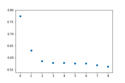
- for문을 돌려서 autocorrelation list에 담기
# lag들을 for문 돌려서 list에 담은 것 -> 전체적으로 조금씩 줄어들고 있는 것을 알 수 있음
autocorrelation=[]
for shift in range(1,10):
    c = np.corrcoef(temps[:-shift], temps[shift:] )[0,1]
    autocorrelation.append( c )
autocorrelation
[OUT] :
[0.7748702165384457,
0.6311194620684836,
0.5863748620126278,
0.5788976133377621,
0.578571574411206,
0.5765484145122557,
0.575928953583158,
0.5695569780397494,
0.5634747178408281]
2. 내장함수 사용
tempDF['Temp'][OUT] :
Date
1981-01-01 20.7
1981-01-02 17.9
1981-01-03 18.8
1981-01-04 14.6
1981-01-05 15.8
...
1990-12-27 14.0
1990-12-28 13.6
1990-12-29 13.5
1990-12-30 15.7
1990-12-31 13.0
Name: Temp, Length: 3650, dtype: float64
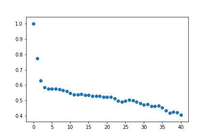
result = acf(tempDF['Temp'])
result
[OUT] :
array([1. , 0.774268 , 0.6302866 , 0.58529312, 0.57774567,
0.57728013, 0.57510412, 0.57437039, 0.56782622, 0.56120131,
0.54668689, 0.53793111, 0.54012564, 0.54247126, 0.53688723,
0.53429917, 0.53043593, 0.52911166, 0.53037444, 0.52280732,
0.52303677, 0.52224579, 0.51426684, 0.49837745, 0.49302665,
0.49946731, 0.50428521, 0.50068173, 0.49157081, 0.48146406,
0.47421245, 0.47568054, 0.46311862, 0.46215585, 0.46630567,
0.45459092, 0.43378232, 0.4203594 , 0.42707505, 0.42196486,
0.4079607 ])시각화
(시계열예측은 non-stationary만 가능)
plt.scatter(range(0,len(autocorrelation)),autocorrelation)
plt.show()
plt.scatter(range(0,len(result)),result)
plt.show() # non-stationary는 점차 감소하는 형태
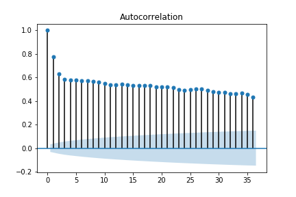
plot_acf(tempDF['Temp']) # 바로 자기상관계수 계산해서 plot으로 그려줌
plt.show() # 점차 감소하는 형태이므로 non-stationary
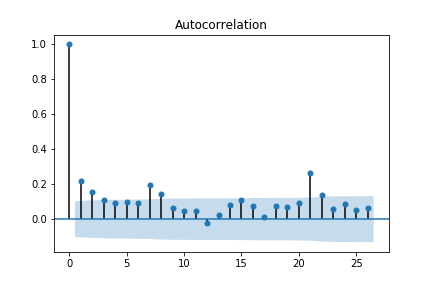
plot_acf(birthDF['Births'])
plt.show() # stationary
plot_acf(airDF['passengers'])
plt.show() # non-stationary는 점차 감소하는 형태

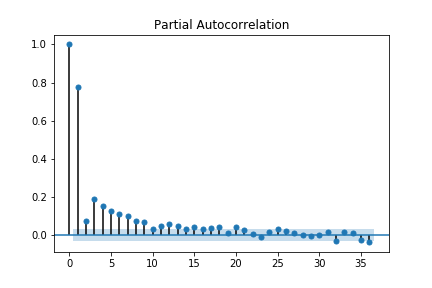
plot_pacf (partial auto correlation function) : 모델 선택용
(실제로는 for문 돌려서 파라미터를 구함)
plot_pacf(tempDF['Temp'])
plt.show()
adfuller 판단지표
검증 조건 ( p-value : 5% 이내면 reject으로 대체가설 선택됨 )
- 귀무가설(H0): non-stationary
- 대체가설 (H1): stationary
result = adfuller(birthDF['Births'])
print(result[0]) # adf(적을수록 : 귀무가설을 기각시킬 확률이 높다)
print(result[1]) # p-value(귀무가설기각:stationary)
[OUT] :
-4.808291253559763
5.243412990149865e-05
result = adfuller(airDF['passengers'])
print(result[0]) # adf(클수록 : 귀무가설을 채택될 확률이 높다)
print(result[1]) # p-value(귀무가설채택:non-stationary)
[OUT] :
0.8153688792060569
0.9918802434376411
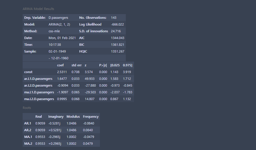
order=(2,1,2) # AR, 차분, MA
model = ARIMA(airDF,order)
rfit = model.fit()
rfit.summary() # AIC가 작을수록 좋음
def arima_aic_check(data, order,sort = 'AIC'):
    order_list = []
    aic_list = []
    bic_lsit = []
    for p in range(order[0]):
        for d in range(order[1]):
            for q in range(order[2]):
                model = ARIMA(data, order=(p,d,q))
                try:
                    model_fit = model.fit()
                    c_order = f'p:{p} d:{d} q:{q}'
                    aic = model_fit.aic
                    bic = model_fit.bic
                    order_list.append(c_order)
                    aic_list.append(aic)
                    bic_list.append(bic)
                except:
                    pass
    result_df = pd.DataFrame(list(zip(order_list, aic_list)),columns=['order','AIC'])
    result_df.sort_values(sort, inplace=True)
    return result_df
arima_aic_check(airDF,[3,3,3])

시계열 예측
rfit.predict(1,10) [OUT] :
1949-02-01 2.531108
1949-03-01 3.350912
1949-04-01 5.221378
1949-05-01 0.789534
1949-06-01 -1.830598
1949-07-01 1.762428
1949-08-01 1.739116
1949-09-01 -0.632656
1949-10-01 -1.201350
1949-11-01 2.076971
Freq: MS, dtype: float64
rfit.predict(1,10, typ='levels') # typ='levels' : 함수 예측 값을 줌[OUT] :
1949-02-01 114.531108
1949-03-01 121.350912
1949-04-01 137.221378
1949-05-01 129.789534
1949-06-01 119.169402
1949-07-01 136.762428
1949-08-01 149.739116
1949-09-01 147.367344
1949-10-01 134.798650
1949-11-01 121.076971
Freq: MS, dtype: float64
rfit.predict('1950-01-01','1950-12-01', typ='levels')[OUT] :
1950-01-01 131.476292
1950-02-01 132.058401
1950-03-01 143.953676
1950-04-01 156.328724
1950-05-01 147.710884
1950-06-01 136.542444
1950-07-01 155.854139
1950-08-01 168.939947
1950-09-01 162.271205
1950-10-01 147.633324
1950-11-01 126.286622
1950-12-01 115.225257
Freq: MS, dtype: float64
train = airDF[:'1960-07-01']
test =  airDF['1960-07-01':]
display(train,test)

preds = rfit.predict('1960-07-01','1960-12-01', typ='levels')
preds
[OUT] :
1960-07-01 553.884401
1960-08-01 599.046866
1960-09-01 555.150224
1960-10-01 458.019193
1960-11-01 421.197229
1960-12-01 378.526383
Freq: MS, dtype: float64
plt.plot(train)
plt.plot(test)
plt.plot(preds,'r--') # test와 preds가 거의 비슷함
plt.show()

# test, pred만 보기
plt.plot(test)
plt.plot(preds,'r--') # test와 preds가 거의 비슷함
plt.show()

미래예측
preds = rfit.predict('1960-07-01','1961-7-01', typ='levels')
preds
[OUT] :
1960-07-01 553.884401
1960-08-01 599.046866
1960-09-01 555.150224
1960-10-01 458.019193
1960-11-01 421.197229
1960-12-01 378.526383
1961-01-01 433.134083
1961-02-01 450.918699
1961-03-01 479.853734
1961-04-01 512.019605
1961-05-01 539.368848
1961-06-01 555.843542
1961-07-01 558.780264
Freq: MS, dtype: float64
plt.plot(train)
plt.plot(test)
plt.plot(preds,'r--') # test와 preds가 거의 비슷함
plt.show()

# test, pred만 보기
plt.plot(test)
plt.plot(preds,'r--')
plt.show()

연습문제
df를 이용하여 acf, adfuller통해서 시계열 stationary여부 확인 후 예측하시오(2001-11-13,2001-11-20)
df = pd.DataFrame([
        ['2001-11-01', 0.998543],
        ['2001-11-02', 1.914526],
        ['2001-11-03', 3.057407],
        ['2001-11-04', 4.044301],
        ['2001-11-05', 4.952441],
        ['2001-11-06', 6.002932],
        ['2001-11-07', 6.930134],
        ['2001-11-08', 8.011137],
        ['2001-11-09', 9.040393],
        ['2001-11-10', 10.097007],
        ['2001-11-11', 11.063742],
        ['2001-11-12', 12.051951],
        ['2001-11-13', 13.062637],
        ['2001-11-14', 14.086016],
        ['2001-11-15', 15.096826],
        ['2001-11-16', 15.944886],
        ['2001-11-17', 17.027107],
        ['2001-11-18', 17.930240],
        ['2001-11-19', 18.984202],
        ['2001-11-20', 19.971603]
    ], columns=['date', 'count'])
df['date'] = pd.to_datetime(df.date, format='%Y-%m-%d')
df = df.set_index('date')
df

Solution
result = acf(df['count'])
result
[OUT] :
array([ 1. , 0.85051096, 0.70111766, 0.55770427, 0.41727086,
0.28272744, 0.15409016, 0.03335875, -0.07545946, -0.17166745,
-0.25369122, -0.32166247, -0.37250429, -0.40465095, -0.41553391,
-0.40615602, -0.37568118, -0.32135199, -0.24323865, -0.13518252])
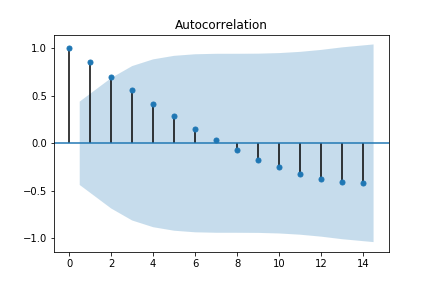
# acf 시각화 -> non-stationary
plot_acf(df['count'])
plt.show()
# adfuller
result = adfuller(df['count'])
print(result[0])
print(result[1]) # p-value(귀무가설 채택:non-stationary)
[OUT] :
-7.573269903543583
2.804546459135478e-11
arima_aic_check(df,[3,3,3]).sort_values # 제일 작은 0,1,1 선택[OUT] :
<bound method DataFrame.sort_values of order AIC
4 p:0 d:1 q:1 -46.510330
10 p:1 d:1 q:0 -46.352253
11 p:1 d:1 q:1 -44.691545
5 p:0 d:1 q:2 -44.595638
16 p:2 d:1 q:0 -44.545073
17 p:2 d:1 q:1 -44.052351
12 p:1 d:1 q:2 -42.796456
3 p:0 d:1 q:0 -41.995440
18 p:2 d:1 q:2 -38.789645
8 p:0 d:2 q:2 -38.039370
14 p:1 d:2 q:1 -37.642422
15 p:1 d:2 q:2 -36.052055
20 p:2 d:2 q:1 -35.851557
7 p:0 d:2 q:1 -33.759830
19 p:2 d:2 q:0 -32.976247
13 p:1 d:2 q:0 -30.849871
6 p:0 d:2 q:0 -18.967009
9 p:1 d:0 q:0 67.211518
2 p:0 d:0 q:2 93.021176
1 p:0 d:0 q:1 111.032398
0 p:0 d:0 q:0 130.860221>
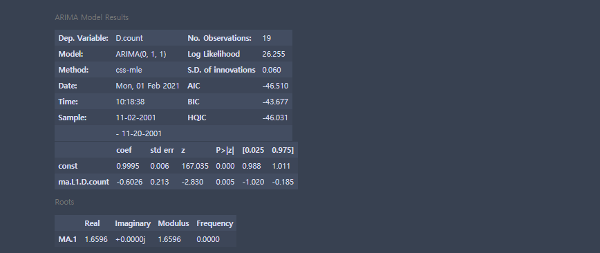
order=(0,1,1) # AR, 차분, MA
model = ARIMA(df,order)
rfit = model.fit()
rfit.summary() # AIC가 작을수록 좋음
train = df[:'2001-11-13']
test =  df['2001-11-13':]
preds = rfit.predict('2001-11-13','2001-11-20', typ='levels')
preds
[OUT] :
2001-11-13 13.050375
2001-11-14 14.054755
2001-11-15 15.066685
2001-11-16 16.078170
2001-11-17 17.024704
2001-11-18 18.025165
2001-11-19 18.986944
2001-11-20 19.985360
Freq: D, dtype: float64
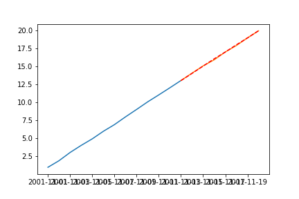
plt.plot(train)
plt.plot(test)
plt.plot(preds,'r--') # test와 preds가 거의 비슷함
plt.show()
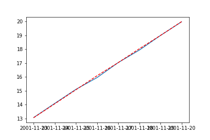
# test, pred만 보기
plt.plot(test)
plt.plot(preds,'r--') # test와 preds가 거의 비슷함
plt.show()
review
- 그래프를 저장하고 싶으면 plt.show() 대신 plt.savefig('img')
'코딩으로 익히는 Python > 모델링' 카테고리의 다른 글
| [Python] 23. PCA(차원축소),T-SNE (11) | 2021.01.26 |
|---|---|
| [Python] 22. Kmeans (0) | 2021.01.26 |
| [Python] 21. SVM(서포트벡터머신) (0) | 2021.01.26 |
| [Python] 20. 나이브베이즈 (0) | 2021.01.26 |
| [Python] 19. MLP : pima-indians 예제 (0) | 2021.01.26 |


